Interview with Zowi: AI for Marine Survey Data at GEOxyz
"We help GEOxyz survey the seabed efficien ...
Published on: July 13, 2018
A few weeks ago, Adrian Rosebrock published an article on multi-label classification with Keras on his PyImageSearch website.
The article describes a network to classify both clothing type (jeans, dress, shirts) and color (black, blue, red) using a single network. The network was trained on a dataset containing images of black jeans, blue dresses, blue jeans, blue shirts, red dresses and red shirts.

The test set contains only a few images, but includes a black dress (there were no black dresses in the training set), which was classified as a black jeans. Adrian’s explanation for this is:
“If your network is trained on examples of both (1) black pants and (2) red shirts and now you want to predict “red pants” (where there are no “red pants” images in your dataset), the neurons responsible for detecting “red” and “pants” will fire, but since the network has never seen this combination of data/activations before once they reach the fully-connected layers, your output predictions will very likely be incorrect (i.e., you may encounter “red” or “pants” but very unlikely both).”
Of course, this made me wonder whether it is possible to design and train a network that is able to fully split the clothing type and color predictions.
First of all, I more or less implemented Adrian’s network, but using the approach François Chollet describes in his excellent Deep Learning with Python book, using data augmentation and a pretrained VGG16 convolutional base, followed by two dense layers. Of course, I got more or less the same results, including the black dress being classified as a black jeans.
Intuitively, I would expect that, given enough images with a (random) single object and a color label, it should be possible to get a quite accurate color prediction, especially because we exclude ambiguous colors and limit our classifier to black, blue and red in this example.
I replaced final the dense layer by one with softmax activation and three one-hot-encoded outputs, and retrained the network using the same procedure. The network started overfitting after a few epochs, even when adding a 90% dropout layer before the each of the two dense layers. I downloaded a few more black dresses and most of them were classified as either blue or red, also indicating that the network is trained to recognise shapes. Given the complexity of the network compared to the problem and the fact that the pretrained VGG16 convolutional base is trained to recognise shapes, this isn’t a big surprise.
So I replaced the VGG16 convolutional base with a much smaller convolutional base, containing only three 2D convolutional layers and three max pooling layers and trained the network from scratch. This small network does an almost perfect job predicting the color, without the ability to recognise shapes.
For the final network, I took the color classifier described above and added a clothing type classifier containing a VGG16 convolutional base (as in the first model), a 25% dropout layer, a dense layer with 256 output nodes and relu activation, another 25% dropout layer and a final dense layer with three output nodes (one-hot encoding for jeans, dress and shirt) with softmax activation.
Using Keras’ functional API, it’s easy to combine both branches in a single network.
To run this notebook, you need Python 3, Keras, TensorFlow (or another backend supported by Keras) NumPy, Pandas and Matplotlib.
Download the training and test images from Adrian Rosebrock’s article at PyImageSearch (and have a look at his article too, his explanations are more detailed than mine). Save the training images in a train subdirectory (keep the color_type subdirectories) and the test (example) images in a test subdirectory.
In [1]:
# More or less standard Python stuff
import datetime
import numpy
import os
import pandas

# Visualisation
%matplotlib inline
import matplotlib.pyplot as plt

# Machine learning
import sklearn
import keras

print(keras.__version__)
Out [1]:
/usr/lib/python3/dist-packages/h5py/__init__.py:36: FutureWarning: Conversion of the second argument of issubdtype from `float` to `np.floating` is deprecated. In future, it will be treated as `np.float64 == np.dtype(float).type`.
from ._conv import register_converters as _register_converters
Using TensorFlow backend.
2.1.6
In [2]:
start_time = datetime.datetime.now()
Define color and type class coding and decoding dictionaries.
In [3]:
base_dir = './train/'
color_classes = {'black': 0, 'blue': 1, 'red': 2}
decode_color_classes = {v: k for k, v in color_classes.items()}
num_color_classes = max(color_classes.values()) + 1
type_classes = {'jeans': 0, 'dress': 1, 'shirt': 2}
decode_type_classes = {v: k for k, v in type_classes.items()}
num_type_classes = max(type_classes.values()) + 1
Store the names of all files in the train subdirectory and their corresponding labels in a Pandas dataframe.
In [4]:
image_files_tuples = []
for dirpath, dirnames, filenames in os.walk(base_dir):
    for filename in filenames:
        filename_full = os.path.join(dirpath, filename)
        labels = os.path.basename(dirpath).split('_')
        color_labels = numpy.zeros((num_color_classes,), numpy.float32)
        color_labels[color_classes[labels[0]]] = 1.
        type_labels = numpy.zeros((num_type_classes,), numpy.float32)
        type_labels[type_classes[labels[1]]] = 1.
        image_files_tuples.append((filename_full, numpy.concatenate((color_labels, type_labels))))
image_files = pandas.DataFrame.from_records(image_files_tuples, columns=['filename', 'targets'])
print('Found ' + str(image_files.shape[0]) + ' annotated images')
Out [4]:
Found 2167 annotated images
Shuffle the images, use 80% for training and the remaining 20% for validation.
In [5]:
image_files_train = sklearn.utils.shuffle(image_files.sample(frac=0.8, random_state=100))
image_files_val = sklearn.utils.shuffle(image_files.drop(image_files_train.index))
print('Using ' + str(image_files_train.shape[0]) + ' training samples')
print('Using ' + str(image_files_val.shape[0]) + ' validation samples')
Out [5]:
Using 1734 training samples
Using 433 validation samples
Use Keras’ image preprocessing functions to create the training and validation data generators. The training data generator uses image data augmentation.
The standard flow_from_directory expects the samples in label subdirectories, but our samples are in label1_label2 subdirectories. Use the flow_from_dataframe function from [https://github.com/keras-team/keras/issues/5152], which gets the filenames and targets from the pandas dataframe constructed earlier.
In [6]:
# From https://github.com/keras-team/keras/issues/5152
def flow_from_dataframe(img_data_gen, in_df, path_col, y_col, **dflow_args):
    base_dir = os.path.dirname(in_df[path_col].values[0])
    print('## Ignore next message from keras, values are replaced anyways')
    df_gen = img_data_gen.flow_from_directory(base_dir, class_mode = 'sparse', **dflow_args)
    df_gen.filenames = in_df[path_col].values
    df_gen.classes = numpy.stack(in_df[y_col].values)
    df_gen.samples = in_df.shape[0]
    df_gen.n = in_df.shape[0]
    df_gen._set_index_array()
    df_gen.directory = '' # since we have the full path
    print('Reinserting dataframe: {} images'.format(in_df.shape[0]))
    return df_gen
Split the 6-element output vector in two 3-element output vectors, needed for our branched model.
In [7]:
def split_outputs(generator):
    while True:
        data = next(generator)
        x = data[0]
        y = numpy.split(data[1], 2, axis=1)
        yield x, y
Initialise the data generators.
In [8]:
train_datagen = keras.preprocessing.image.ImageDataGenerator(rescale=1./255,
                                                             rotation_range=10,
                                                             width_shift_range=0.2,
                                                             height_shift_range=0.2,
                                                             shear_range=0.1,
                                                             zoom_range=0.2,
                                                             horizontal_flip=True)
validation_datagen = keras.preprocessing.image.ImageDataGenerator(rescale=1./255)

train_generator = split_outputs(flow_from_dataframe(train_datagen, image_files_train, 'filename', 'targets',
                                                    target_size=(160, 128), batch_size=20))
validation_generator = split_outputs(flow_from_dataframe(validation_datagen, image_files_val, 'filename', 'targets',
                                                         target_size=(160, 128), batch_size=20))
Out [8]:
## Ignore next message from keras, values are replaced anyways
Found 0 images belonging to 0 classes.
Reinserting dataframe: 1734 images
## Ignore next message from keras, values are replaced anyways
Found 0 images belonging to 0 classes.
Reinserting dataframe: 433 images
Create sequential models for both the color and type classifier and create a combined single-input multi-output model using Keras’ functional API.
In [9]:
input_images = keras.Input(shape=(160, 128, 3), dtype='float32', name='images')

color_model = keras.models.Sequential()
color_model.add(keras.layers.Conv2D(32, (11, 11), strides=(4, 4), activation='relu', input_shape=(160, 128, 3),
                                    padding='same'))
color_model.add(keras.layers.MaxPooling2D((2, 2)))
color_model.add(keras.layers.Conv2D(64, (3, 3), activation='relu', padding='same'))
color_model.add(keras.layers.MaxPooling2D((2, 2)))
color_model.add(keras.layers.Conv2D(64, (3, 3), activation='relu', padding='same'))
color_model.add(keras.layers.MaxPooling2D((2, 2)))
color_model.add(keras.layers.Flatten())
color_model.add(keras.layers.Dropout(0.5))
color_model.add(keras.layers.Dense(128, activation='relu'))
color_model.add(keras.layers.Dropout(0.5))
color_model.add(keras.layers.Dense(3, activation='softmax'))
color_model.name = 'color'

color_output = color_model(input_images)

conv_base = keras.applications.VGG16(weights='imagenet', include_top=False, input_shape=(160, 128, 3))
conv_base.trainable = False
type_model = keras.models.Sequential()
type_model.add(conv_base)
type_model.add(keras.layers.Flatten())
type_model.add(keras.layers.Dropout(0.25))
type_model.add(keras.layers.Dense(256, activation='relu'))
type_model.add(keras.layers.Dropout(0.25))
type_model.add(keras.layers.Dense(3, activation='softmax'))
type_model.name = 'type'

type_output = type_model(input_images)

model = keras.models.Model(input_images, [color_output, type_output])
Compile the model. Use categorical crossentropy losses for both outputs.
In [10]:
model.compile(loss={'color': 'categorical_crossentropy', 'type': 'categorical_crossentropy'},
              optimizer=keras.optimizers.RMSprop(lr=1e-4),
              metrics=['accuracy'])
model.summary()
Out[10]:
__________________________________________________________________________________________________
Layer (type) Output Shape Param # Connected to
==================================================================================================
images (InputLayer) (None, 160, 128, 3) 0
__________________________________________________________________________________________________
color (Sequential) (None, 3) 231427 images[0][0]
__________________________________________________________________________________________________
type (Sequential) (None, 3) 17337155 images[0][0]
==================================================================================================
Total params: 17,568,582
Trainable params: 2,853,894
Non-trainable params: 14,714,688
__________________________________________________________________________________________________
Train the color model and the dense layers of the type model for 10 epochs. The pretrained weights of the VGG16 convolutional base are locked because otherwise the larger errors caused by the random initialisation would destroy the pretrained weights.
In [11]:
history = model.fit_generator(train_generator,
                              steps_per_epoch=100,
                              epochs=10,
                              validation_data=validation_generator,
                              validation_steps=20)
Out [11]:
Epoch 1/10
/usr/lib/python3/dist-packages/PIL/Image.py:914: UserWarning: Palette images with Transparency expressed in bytes should be converted to RGBA images
'to RGBA images')
100/100 [==============================] - 82s 816ms/step - loss: 1.1962 - color_loss: 0.7727 - type_loss: 0.4236 - color_acc: 0.6819 - type_acc: 0.8385 - val_loss: 0.5379 - val_color_loss: 0.4271 - val_type_loss: 0.1109 - val_color_acc: 0.8375 - val_type_acc: 0.9600
Epoch 2/10
100/100 [==============================] - 36s 360ms/step - loss: 0.6353 - color_loss: 0.4182 - type_loss: 0.2170 - color_acc: 0.8284 - type_acc: 0.9133 - val_loss: 0.3551 - val_color_loss: 0.2698 - val_type_loss: 0.0853 - val_color_acc: 0.8346 - val_type_acc: 0.9644
Epoch 3/10
100/100 [==============================] - 36s 357ms/step - loss: 0.4627 - color_loss: 0.2974 - type_loss: 0.1653 - color_acc: 0.8754 - type_acc: 0.9380 - val_loss: 0.2047 - val_color_loss: 0.1551 - val_type_loss: 0.0496 - val_color_acc: 0.9644 - val_type_acc: 0.9796
Epoch 4/10
100/100 [==============================] - 35s 353ms/step - loss: 0.3414 - color_loss: 0.2139 - type_loss: 0.1275 - color_acc: 0.9235 - type_acc: 0.9558 - val_loss: 0.2142 - val_color_loss: 0.1448 - val_type_loss: 0.0694 - val_color_acc: 0.9491 - val_type_acc: 0.9644
Epoch 5/10
100/100 [==============================] - 35s 349ms/step - loss: 0.2863 - color_loss: 0.1588 - type_loss: 0.1275 - color_acc: 0.9388 - type_acc: 0.9521 - val_loss: 0.2510 - val_color_loss: 0.1945 - val_type_loss: 0.0566 - val_color_acc: 0.9186 - val_type_acc: 0.9746
Epoch 6/10
100/100 [==============================] - 36s 357ms/step - loss: 0.2381 - color_loss: 0.1240 - type_loss: 0.1141 - color_acc: 0.9545 - type_acc: 0.9573 - val_loss: 0.1209 - val_color_loss: 0.0694 - val_type_loss: 0.0514 - val_color_acc: 0.9644 - val_type_acc: 0.9796
Epoch 7/10
100/100 [==============================] - 35s 355ms/step - loss: 0.2201 - color_loss: 0.1153 - type_loss: 0.1048 - color_acc: 0.9528 - type_acc: 0.9628 - val_loss: 0.0924 - val_color_loss: 0.0535 - val_type_loss: 0.0389 - val_color_acc: 0.9796 - val_type_acc: 0.9847
Epoch 8/10
100/100 [==============================] - 34s 343ms/step - loss: 0.1864 - color_loss: 0.0907 - type_loss: 0.0956 - color_acc: 0.9680 - type_acc: 0.9650 - val_loss: 0.1161 - val_color_loss: 0.0486 - val_type_loss: 0.0674 - val_color_acc: 0.9746 - val_type_acc: 0.9695
Epoch 9/10
100/100 [==============================] - 35s 351ms/step - loss: 0.1625 - color_loss: 0.0782 - type_loss: 0.0843 - color_acc: 0.9725 - type_acc: 0.9655 - val_loss: 0.1382 - val_color_loss: 0.0885 - val_type_loss: 0.0497 - val_color_acc: 0.9695 - val_type_acc: 0.9796
Epoch 10/10
100/100 [==============================] - 36s 360ms/step - loss: 0.1504 - color_loss: 0.0732 - type_loss: 0.0772 - color_acc: 0.9750 - type_acc: 0.9695 - val_loss: 0.1227 - val_color_loss: 0.0440 - val_type_loss: 0.0787 - val_color_acc: 0.9796 - val_type_acc: 0.9695
Save the model.
In [12]:
model.save('clothing_type_and_color_classifier_v3_1.h5')
Plot the training and validation accuracy and loss
In [13]:
def plot_training_history(history):
    color_acc = history.history['color_acc']
    val_color_acc = history.history['val_color_acc']
    color_loss = history.history['color_loss']
    val_color_loss = history.history['val_color_loss']
    type_acc = history.history['type_acc']
    val_type_acc = history.history['val_type_acc']
    type_loss = history.history['type_loss']
    val_type_loss = history.history['val_type_loss']
    epochs = range(len(color_acc))

    plt.figure(figsize=(15, 6))
    plt.subplot(1, 2, 1)
    plt.plot(epochs, color_acc, 'bo', label='Color training acc')
    plt.plot(epochs, val_color_acc, 'b', label='Color validation acc')
    plt.plot(epochs, type_acc, 'ro', label='Type training acc')
    plt.plot(epochs, val_type_acc, 'r', label='Type validation acc')
    plt.title('Training and validation accuracy')
    plt.legend()

    plt.subplot(1, 2, 2)
    plt.plot(epochs, color_loss, 'bo', label='Color training loss')
    plt.plot(epochs, val_color_loss, 'b', label='Color validation loss')
    plt.plot(epochs, type_loss, 'ro', label='Type training loss')
    plt.plot(epochs, val_type_loss, 'r', label='Type validation loss')
    plt.title('Training and validation loss')
    plt.legend()

    plt.show()
In [14]:
plot_training_history(history)
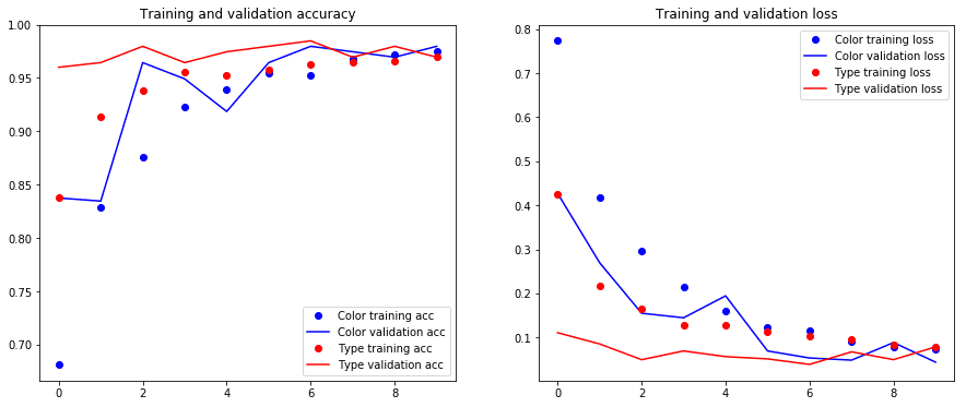
Unlock the last layer of the convolutional base (block5_*), recompile the model (necessary because we changed the model) and train for another 5 epochs, focusing on the type classification. Since the dense layers on top are more or less trained, the gradients will be lower and the weights in the top layer of the convolutional base will be improved for our application. Save the model and plot the training and validation accuracy and loss.
In [15]:
conv_base.trainable = True

set_trainable = False
for layer in conv_base.layers:
    if layer.name == 'block5_conv1':
        set_trainable = True
    if set_trainable:
        layer.trainable = True
    else:
        layer.trainable = False
In [16]:
model.compile(loss={'color': 'categorical_crossentropy', 'type': 'categorical_crossentropy'},
              loss_weights={'color': 0.1, 'type': 1.},
              optimizer=keras.optimizers.RMSprop(lr=1e-5),
              metrics=['accuracy'])

model.summary()
Out [16]:
__________________________________________________________________________________________________
Layer (type) Output Shape Param # Connected to
==================================================================================================
images (InputLayer) (None, 160, 128, 3) 0
__________________________________________________________________________________________________
color (Sequential) (None, 3) 231427 images[0][0]
__________________________________________________________________________________________________
type (Sequential) (None, 3) 17337155 images[0][0]
==================================================================================================
Total params: 17,568,582
Trainable params: 9,933,318
Non-trainable params: 7,635,264
__________________________________________________________________________________________________
In [17]:
history = model.fit_generator(train_generator,
                              steps_per_epoch=100,
                              epochs=5,
                              validation_data=validation_generator,
                              validation_steps=20)
Out [17]:
Epoch 1/5
66/100 [==================>...........] - ETA: 11s - loss: 0.0910 - color_loss: 0.0553 - type_loss: 0.0855 - color_acc: 0.9871 - type_acc: 0.9712
/usr/lib/python3/dist-packages/PIL/Image.py:914: UserWarning: Palette images with Transparency expressed in bytes should be converted to RGBA images
'to RGBA images')
100/100 [==============================] - 39s 395ms/step - loss: 0.0766 - color_loss: 0.0516 - type_loss: 0.0714 - color_acc: 0.9865 - type_acc: 0.9765 - val_loss: 0.0431 - val_color_loss: 0.0418 - val_type_loss: 0.0389 - val_color_acc: 0.9796 - val_type_acc: 0.9847
Epoch 2/5
100/100 [==============================] - 36s 356ms/step - loss: 0.0702 - color_loss: 0.0631 - type_loss: 0.0639 - color_acc: 0.9780 - type_acc: 0.9770 - val_loss: 0.0328 - val_color_loss: 0.0439 - val_type_loss: 0.0284 - val_color_acc: 0.9822 - val_type_acc: 0.9847
Epoch 3/5
100/100 [==============================] - 35s 351ms/step - loss: 0.0367 - color_loss: 0.0532 - type_loss: 0.0314 - color_acc: 0.9823 - type_acc: 0.9910 - val_loss: 0.0262 - val_color_loss: 0.0496 - val_type_loss: 0.0212 - val_color_acc: 0.9771 - val_type_acc: 0.9924
Epoch 4/5
100/100 [==============================] - 36s 356ms/step - loss: 0.0503 - color_loss: 0.0509 - type_loss: 0.0452 - color_acc: 0.9825 - type_acc: 0.9860 - val_loss: 0.0134 - val_color_loss: 0.0420 - val_type_loss: 0.0092 - val_color_acc: 0.9822 - val_type_acc: 0.9975
Epoch 5/5
100/100 [==============================] - 36s 358ms/step - loss: 0.0462 - color_loss: 0.0607 - type_loss: 0.0402 - color_acc: 0.9793 - type_acc: 0.9860 - val_loss: 0.0207 - val_color_loss: 0.0305 - val_type_loss: 0.0177 - val_color_acc: 0.9873 - val_type_acc: 0.9949
In [18]:
type_model.save('clothing_type_and_color_classifier_v3_2.h5')
In [19]:
plot_training_history(history)
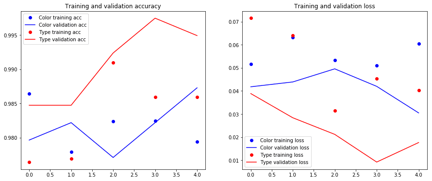
Finally, test the model on the test samples.
In [20]:
test_dir = './test'

filenames_full = []
for dirpath, dirnames, filenames in os.walk(test_dir):
    for filename in filenames:
        filenames_full.append(os.path.join(dirpath, filename))

rows = (len(filenames_full) - 1) // 4 + 1
plt.figure(figsize=(15, 5 * rows))
for index, filename_full in enumerate(filenames_full):
    plt.subplot(rows, 4, index + 1)
    test_image = keras.preprocessing.image.load_img(filename_full, target_size=(160, 128))
    test_input = keras.preprocessing.image.img_to_array(test_image) * (1. / 255)
    test_input = numpy.expand_dims(test_input, axis=0)
    plt.imshow(test_image)
    plt.axis('off')
    prediction = model.predict(test_input)
    color_name = decode_color_classes[numpy.argmax(prediction[0][0, :])]
    type_name = decode_type_classes[numpy.argmax(prediction[1][0, :])]
    plt.title(color_name + ' ' + type_name)

In [21]:
stop_time = datetime.datetime.now()

print('Executing the notebook took', (stop_time - start_time).total_seconds(), 'seconds')
Out [21]:
Executing the notebook took 589.489566 seconds