Interview with Frank Dekervel: Agentic AI, Applied
"Agentic AI turns the knowledge worker fro ...
Published on: April 7, 2020
Last year, Kapernikov embarked upon a new project with Infrabel’s Lidar data: the detection of catenary cables and their intersections. Even though the segmentation and classification of 3D structures in Lidar data is an interesting subject in itself, the context of railway data clearly shows how the identification of the points that form a cable can serve as a great predictive maintenance tool.
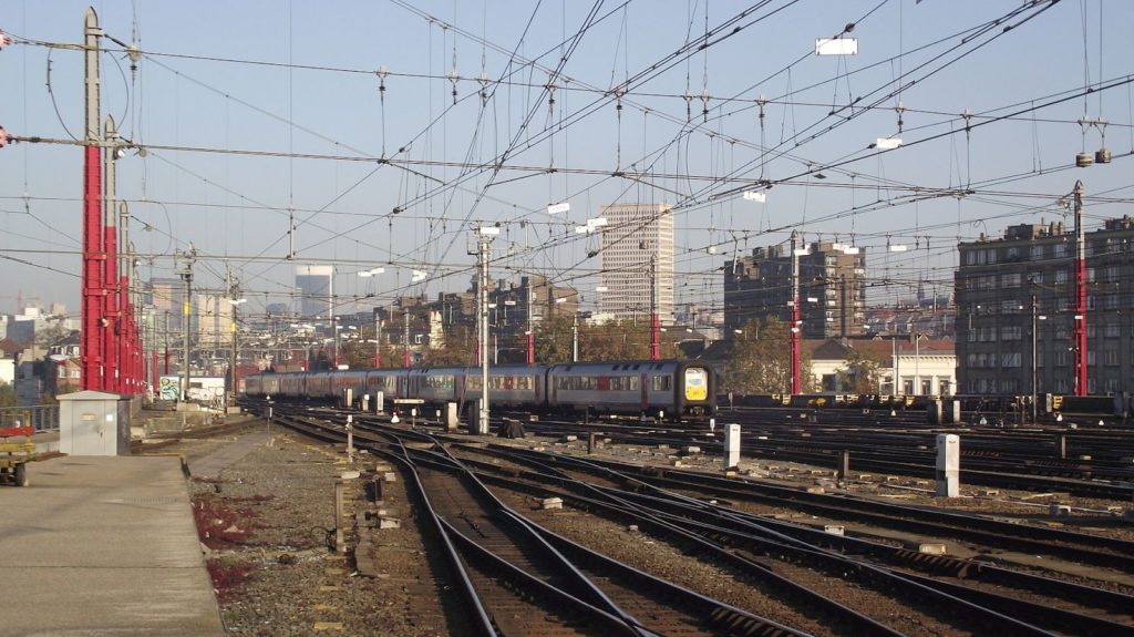
The catenary and contact wires are an essential component of the railway system, since they bring electric power to the trains through the pantographs. These cables usually consist of conductive materials such as aluminum or copper. However, even though metallic cables are ideal for the electrification of the railway, they can be significantly affected by the changes in temperature throughout the year.
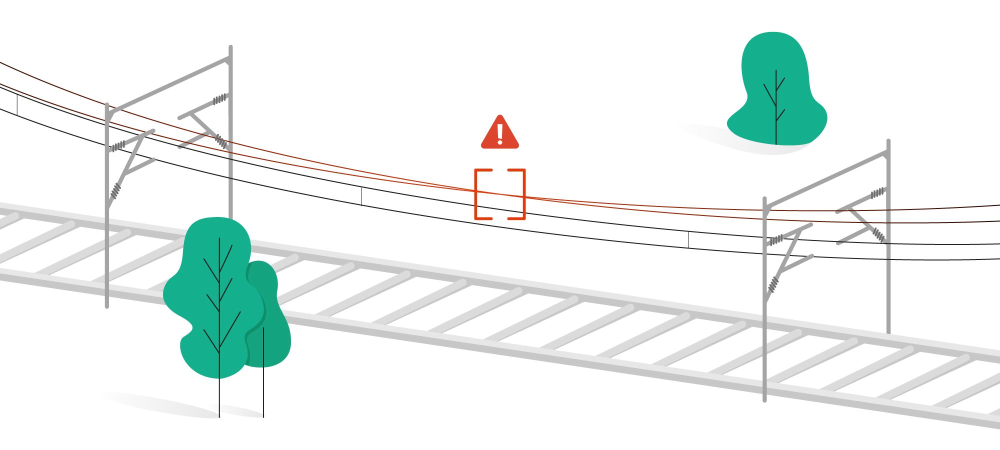
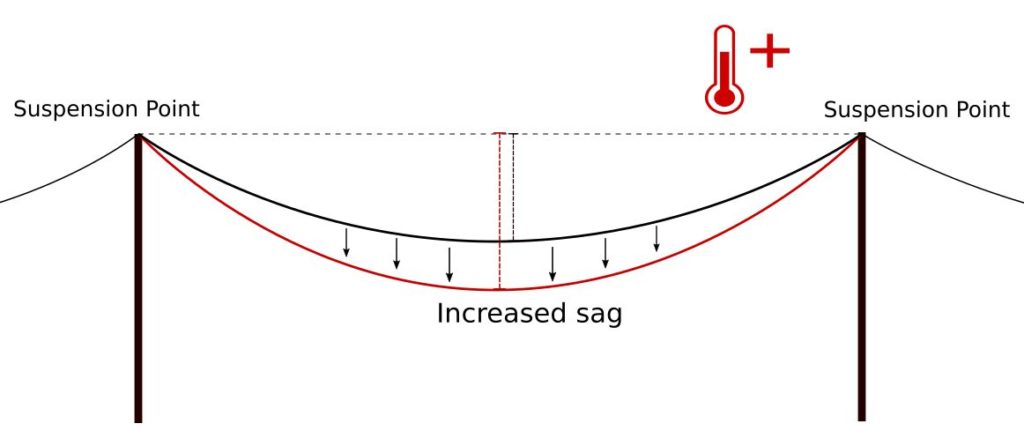
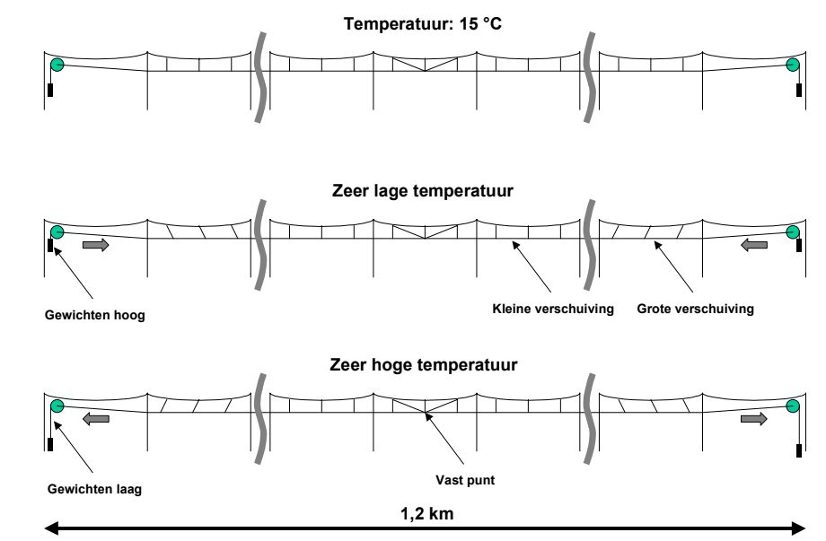
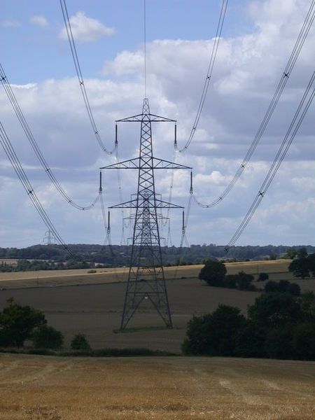
During the summer, high temperatures can stress the railways in many ways, but especially in the case of catenary cables without a mechanical tensioning system, heat can result in their expansion and in the subsequent loosening of their tension, causing them to sag excessively [Fig.1-2]. The increase of the sag is problematic in the locations where the power-carrying cables are crisscrossing and might touch each other, resulting in sparks and operation problems.
To avoid such incidents, the problem should be dealt with within a predictive maintenance framework: possible intersections points should be detected on time and the distance between the crossing cables should act as a measure of their danger level. Currently, cables that get significantly close are normally identified manually, and if it is deemed necessary, they are covered with isolation material. However, Infrabel’s Lidar data offers a source of information that can support the automatization of this process by identifying dangerous intersections without a field visit. This results in a predictive framework for avoiding heat related problems.
In a similar fashion as we did for the vegetation detection project, we decided to use Infrabel’s mobile Lidar data to first detect the cables and then identify possible intersections points where the cables are crossing each other.
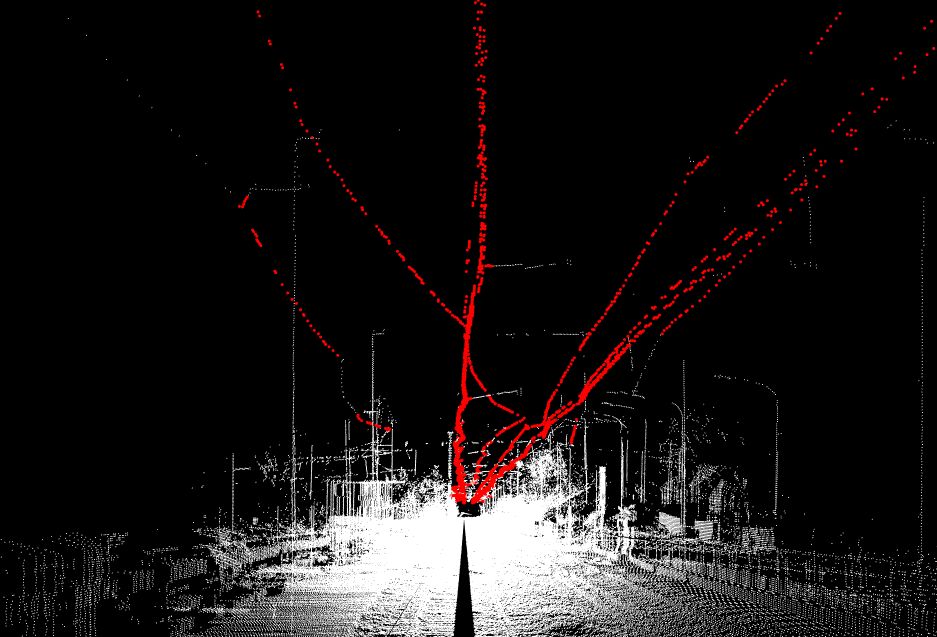
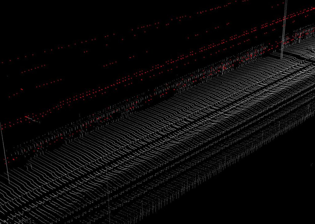
Infrabel’s Lidar dataset, as many mobile Lidar datasets, is characterised by variable density and precision. In the case of the cables, they are usually presented as a single line of points; the ones right above the Lidar having a more consistent density than the ones further away. It is also quite common that the continuity of a cable is interrupted by gaps. [Fig.3]
To tackle the sparse and non-continuous structure of the cables, we initially tried state-of-the-art point cloud semantic segmentation techniques. However, we soon encountered the problem that such methods are good at labelling each point with a class, but they are not the best at identifying and segmenting individual cables. For that reason, we decided to tackle the problem with an algorithmic approach and to employ a typical computer vision method used to detect structures. We based our method on a variation of the RANSAC algorithm.
RANSAC [1] stands for Random Sample Consensus. It is an algorithm that is used to fit a model to data that contain noise. In contrast to classical techniques for parameter estimation, which optimize the fit of a model based on all data, RANSAC assumes that the data consist of both inliers (data points that fit the model) and outliers (data points that do not fit the model), and tries to distinguish between them.
Its method is simple. As a starting point, a random subset of data samples is selected and it is used to estimate the model parameters. Then the data samples that fall within an allowed tolerance distance from the model are considered as inliers. The process is repeated many times and the number of inliers serves as the quality measure of each model. The model that achieves the most inliers is the one that best describes the dataset and is used to reject the outliers. [Fig.4]
PCL, a C++ library used for point cloud processing offers some implementations of RANSAC and a selection of models in order to detect spheres, planes, cylinders or lines in point clouds. We decided to create a variation of the existing RANSAC method which could be applied to detect parabolas.
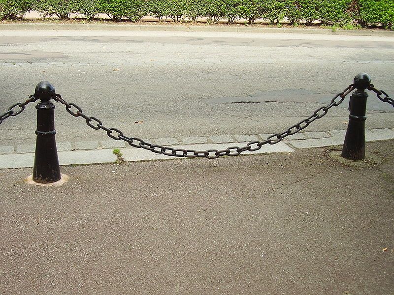
Catenary cables, as their name suggests, can be geometrically described by catenary curves, shapes that correspond to any flexible wire suspended from two points and acted upon by gravity [Fig.5].
Although catenaries are similar to parabolas, they do have a different shape. There are very quick ways to fit a parabola through a bunch of points though, such as polynomial regression. Techniques to fit a catenary tend to be considerably more expensive in terms of computational resources, and as a result, RANSAC would not be that suitable to detect the catenary structures. To tackle this, we decided to use a parabola instead of a catenary curve as our parametric model for RANSAC.
In our data, the cables have relatively small amounts of sag compared to the distance they overspan. Under such conditions, the catenary curve can be very neatly approximated by a parabola, namely its second-order Taylor approximation at the point of minimal height [Fig.6]. For our data, the difference between the catenary and this parabola would typically result in errors less than 1 mm, which seems more than enough justification to use parabolas instead of true catenaries as the underlying model. This is also illustrated by the following plot of a catenary where the sag/overspan ratio is under 1/20, together with its approximating parabola. (N.B. the horizontal and vertical scales are not identical.)

Our implementation for detecting 3D parabolas was based on the existing model implementations. In order to do that, we created a subclass of the SampleConsensusModel class. We set the minimum number of samples to 3, as we need at least 3 points to define a parabola, and we set the number of model parameters to 6. The 3 first are the coordinates of the parabola’s vertex point, the next 2 are the direction vector that gives us the orientation of the parabola in space and the last on is the quadratic coefficient (c), the term that causes the ends of the parabola to curve upwards or downwards.
Then we implemented the necessary functions:
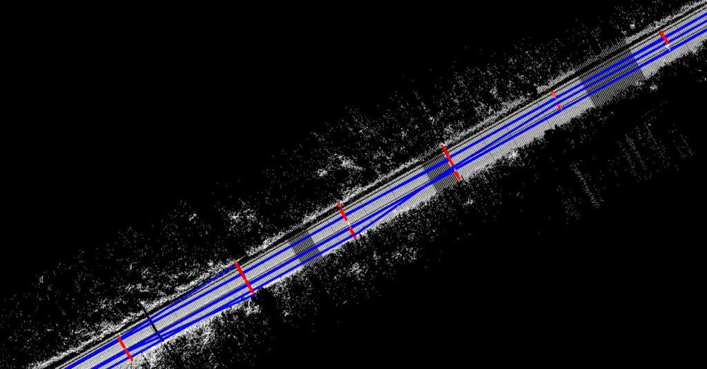
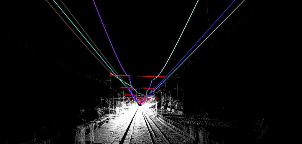
The cable structure is often more complicated than detecting a sequence of points in the shape of parabola. To tackle this complexity, we decided on including a routine for detecting traverses in a pipeline, i.e. the horizontal structures onto which the cables are suspended. RANSAC is used for the traverse detection as well, but with a model that detects horizontal lines. After the traverses have been detected, the cable detection process is applied on point cloud pieces between consecutive traverses. In that way, we can limit the input cloud to a few well formed parabolas [Fig.7-9]. In the final step of the pipeline, the possible intersection points between the detected cables are identified. As shown in the video below, the distance between the cables at the points of intersection helps us to predict if the pair of cables poses a threat to the operation of the railway during summer months.
[1] M. A. Fischler, R. C. Bolles. Random Sample Consensus: A Paradigm for Model Fitting with Applications to Image Analysis and Automated Cartography. Comm. of the ACM, Vol 24, pp 381-395, 1981.