CopernNet : Point Cloud Segmentation using ActiveSampling Transformers
In the dynamic field of railway maintenance, accurate data is critical. From ensuring the health of ...


Published on: December 2, 2018

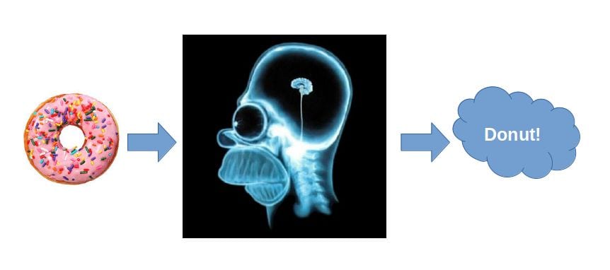
Computer Vision is the subfield of artificial intelligence which tries to imitate the human vision capabilities. And by “human vision”, we do not merely mean the eyes or the ability to see images – it is not as trivial as simply taking a picture with your phone. The purpose is not to imitate just sight, but actually to imitate perception – the ability of humans to make sense of what they see. [Fig. 1]
If we parallelize the human and computer vision systems, we can say that both consist of a sensor and an interpreter. When it comes to sensors, cameras are most often considered the equivalent of the eyes for a computer vision system. In reality, cameras are only a part of a wide range of hardware that are used to capture information about the real world. Just to name a few, there are RGB, monochrome or even hyperspectral cameras but also distance sensors, laser scanners, radars, etc.
Depending on the application, different combinations of these sensors can be selected. In the case of interpreters, a combination of hardware (computers, CPUs etc) and software (algorithms) is used to imitate the human brain and interpret the input data from the sensor. In this article, we will focus not so much on the hardware part of computer vision, but rather on the methods that are used to extract information from images.
As a field, computer vision emerged in the late 60’s and developed almost parallely with the AI field. The first low-level tasks, such as color segmentation or edge detection, were already applied in the early days of the field and formed the foundation of many modern computer vision applications. However, by the 80’s, computer reasoning was still far from achieved and the scientific world generally agreed that the problem was not as trivial as they initially thought it was. Scientists quickly came to realise that tasks that are easily or even unconsciously done by humans are very difficult for a computer and the opposite.
This principle, commonly known as Moravec’s paradox, was first formulated by the computer scientist Hans Moravec and it basically highlights that you can make Deep Blue beat Kasparov in chess, but you cannot easily give a computer the capabilities of a toddler to recognise their parents, to find their favourite toy in the room, to walk without bumping (too much) onto walls. The difficulties of the computer vision field specifically, but also the AI field in general, have led to two periods of reduced funding and interest in research in the late 70’s and the early 90’s, known as “AI winters”.
However, since the mid-90s, the field has seen an increase in interest with the widespread use of machine learning and the first industrial applications. In the past decade, the introduction of deep learning has reinforced the interest in the field, intensifying the talk about an “AI spring”.
But why is it so challenging? Well, first of all, it is not very easy to imitate something that you do not completely understand. Human cognition is not yet completely deciphered and computer vision is highly dependent on the discoveries of the neuroscience field. But even for the part of cognition that we do understand, reproducing the same abilities in a machine is not an easy task.
The perception of humans comes with a pre-existing knowledge about the object and the geometry: seeing a 2D image, one can easily distinguish between foreground and background objects and effortlessly recognise an object even if it is subject to occlusions, background clutter or deformations. But computers cannot distinguish easily between object pixels and background pixels. Or in case of a many-to-one relation between image and label, they cannot easily tell one object from another. More importantly, they cannot extract higher-level information from images: they cannot recognise the emotion on a face or the action being performed in a scene.
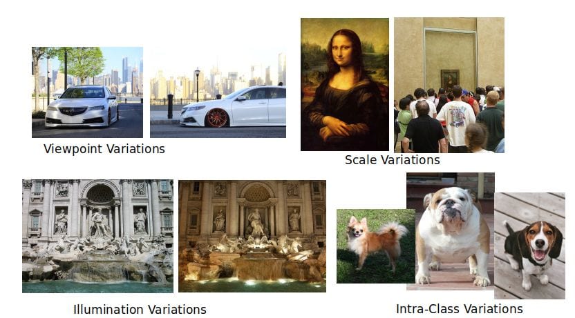
Additionally, there is also the issue of data representation. Humans have ways to organise their knowledge in order to reason and reach conclusions about what they see. For example, upon seeing an image of a zebra, they can identify it based on its attributes, like its 4 legs or its stripes, but also because it resembles a horse and it is standing in the savannah. In the case of computers, they perceive digital images not as something continuous with semantic information, but just as a series of discrete numerical values. This data representation does not allow for an easy extraction of higher-level knowledge and hinders the comparison between images of similar things. Computer vision systems are usually very sensitive to variations such as scale, viewpoint or illumination and intra-class differences [Fig.2].
Feature extraction together with Bag-of-Visual-Words models formed the basis of many image recognition methods of the 2000’s. There are various different feature extraction methods used to extract information either from the whole image (global) or just from image patches (local). A feature extractor usually identifies an image structure based on the intensity values and translates it into a vector of values which can serve a descriptive data representation based on which two images can be compared. These vectors usually have a fixed length and they are used to find correspondences between images by comparing the distances between vectors.
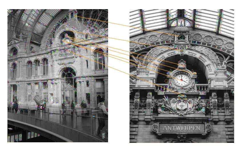
A global feature extractor directly extracts a description for the whole image. However, when it comes to local feature extractors, they usually include an extra step or feature detection before the extraction of features. A feature detector identifies points of interest in an image, i.e. corners, edges, blobs etc. The purpose of the feature detection is to reduce the computational time required to extract features. Instead of pixel by pixel application, the subsequent step of feature description is only applied to the points of interest. Hence, one important characteristic of feature detection algorithms is its repeatability: the ability to find the same points of interest in two images [Fig.3].
Different descriptors were developed to tackle different kind of variations and deformations. One of the most famous feature descriptors, SIFT (shift invariant feature transform), extracts features based on local gradient orientations around points of interest and it is rotation and scale invariant. Other famous local feature extractors include SURF, which is considered a faster alternative to SIFT, MSER which is affine-invariant, DaLI which is invariant to illumination changes and deformations, DAISY, BRIEF, FREAK, etc. Depending on the application, different sets of descriptors can be used.
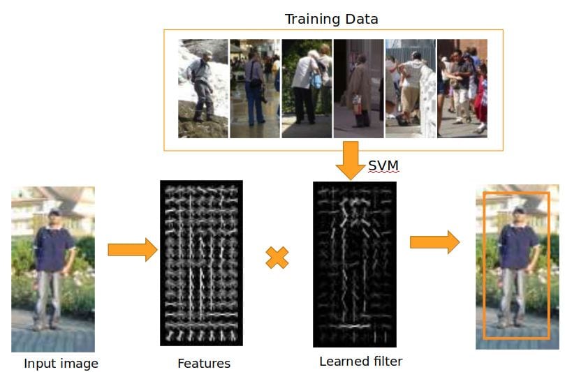
Machine learning is a way of “teaching” computers to make predictions without being explicitly programmed. Similarly to how humans learn, computers can be taught by example. Based on the availability and the amount of labeled data, learning methods are categorized as supervised, semi-supervised or unsupervised. A typical machine learning pipeline for computer vision application starts with feature extraction on the training set. The features are then used as an input in a classifier (ie SVM, KNN, ANN ect) and, following a training step, a model is created. This model can receive new, not previously used images, process them and make predictions about their label based on the knowledge extracted from the training set [Fig. 4].
Unless you live under a rock, you have heard about Deep Learning. You might have heard, for example, Google’s AlphaGo beating the best player in the world or you might have heard about – the many- autonomous driving applications. Or, in the field of medicine, you might have heard that AI performs better than doctors in the diagnosis of melanoma. Deep learning is a method that has been known for 20 years already, with the introduction of Convolutional Neural Networks (CNNs) by Yann LeCun in 1989. However, only in the last decade did the method deep learning see real a surge of interest, especially after 2012, with the introduction of AlexNet by Alex Krizhevsky, a work that built upon CNNs.
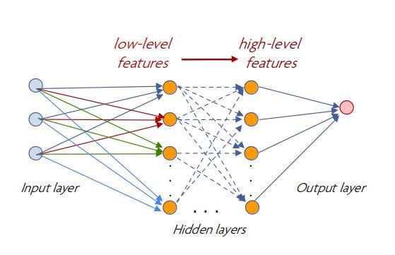
A deep neural network consists of a -usually large- number of hidden layers. The layers are also known as convolutional layers, since they use convolution filters in order to extract features. In the first layers, the extracted features are very “low-level” comprising of edges or blobs, but gradually, in the consequent layers, the features move to higher levels of abstraction. At the final step, the network gives probabilities about the possible classes the input image is more likely to belong to. These probabilities are tuned by back-propagation, a method used to gradually update the intrinsic weights and biases of the network based on the error of the predicted classes. Using back propagation, the network is trained based on labeled data until the final predictions are accurate enough.
The good thing about this method, apart from the astonishing results, is that feature extraction is no longer needed: the network extracts its own features. The bad thing about deep learning is that it requires enormous amounts of data in order to train your network – and, in fact, annotated data. Indicatively, ImageNet, the image data set that made possible the training of CNNs, consists of more than 14 millions of images classified in about 22.000 classes.
Data sets of this size are very difficult to collect and even more difficult to annotate. Services as Mechanical Turk have significantly assisted the annotation process, however the problem still remains where the data is limited. Interestingly, deep learning can also be applied on smaller data sets with a technique called transfer learning. This technique, also know as domain adaptation, instead of training a model from scratch, uses pre-trained models as a starting point which is modified to work also in a thematically different data set. Transfer learning minimises the requirements in data but also in processing power, since less training is required and, thus, it has enabled application in fields like Medicine, Archaeology and Industry.