Interview with Stef: LiDAR innovations at Infrabel
"It's rewarding to start with a raw point ...
Published on: January 24, 2019

The robot_localization package is a collection of non-linear state estimators for robots moving in 3D (or 2D) space. (package summary – documentation)
Each of the state estimators can fuse an arbitrary number of sensors (IMUs, odometers, indoor localization systems, GPS receivers…) to track the 15 dimensional (x, y, z, roll, pitch, yaw, x˙, y˙, z˙, roll˙, pitch˙, yaw˙, x¨, y¨, z¨) state of the robot.
The documentation of the robot_localization package is quite clear once you know how it works. However, it lacks a hands-on tutorial to help you with your first steps. There are some great examples on how to set up the robot_localization package, but they require good working hardware. This tutorial tries to bridge the gap, using the turtlesim package as a virtual robot. We will add a virtual odometer and a virtual (LiDAR) positioning system (both with a configurable systematic and random error) to the turtlesim robot and estimate its location by using the robot_localization package. Of course, you will need a system with ROS (the tutorial is developed and tested with ROS (1) Melodic Morenia on Ubuntu 18.04 Bionic Beaver) and a keyboard to control our turtlesim robot, but that’s it.
I suppose you have some basic knowledge on ROS (if not, start with the beginner level tutorials) and tf2 (if not, read the learning tf2 tutorials) and you understand basic C++ code. You can use robot_localization from Python too, but I implemented the virtual sensors in C++.
To understand how robot_localization works, we should first have a look at REP 103 “Standard Units of Measure and Coordinate Conventions” and REP 105 “Coordinate Frames for Mobile Platforms” which describe the coordinate system conventions used in ROS in general and for mobile robots in particular.
REP 105 defines the tf2 coordinate frame tree for mobile robots:
(earth) → map → odom → base_link
At the lowest level in this graph, the base_link is rigidly attached to the mobile robot’s base. The base_link frame can be attached in any arbitrary position or orientation, but REP 103 specifies the preferred orientation of the frame as X forward, Y left and Z up.
The odom frame is a (more or less) world-fixed frame. The pose of the mobile robot in the odom frame can drift over time, making it useless as a long-term global reference. However, the pose of the robot in the odom frame is guaranteed to be continuous, making it suitable for tasks like visual servoing.
The map frame is a world-fixed frame. The pose of the mobile robot in the map frame should not drift over time, but can change in discrete jumps. This makes the map frame perfect as a long-term global reference, but the discrete jumps make local sensing and acting difficult. REP 103 specifies the preferred orientation as X east, Y north and Z up, but in known structured environments aligning the X and Y axes with the environment is more useful (which is also acknowledged in REP103).
The earth frame at the highest level in the graph is often not necessary, but it can be defined to link different map frames to allow interaction between mobile robots in different map frames or to allow robots to move from one map frame to another. We don’t use the earth frame in this tutorial.
The tree, especially the construction with the map and odom frames, may look counterintuitive at first. It should make sense if you think about the odom → base_link transform as the (best) estimate of the mobile robot’s pose based on continuous sensors (IMUs, odometry sources, open-loop control…) only. The map → odom transform includes the non-continuous sensors (GPS, LiDAR based positioning system…) and models the jumps in the estimated position of the mobile robot, keeping the odom → base_link transform continuous. This approach provides a drift-free but non-continuous (map → base_link) as well as a continuous but drifting (odom → base_link) pose estimation of the mobile robot.
The robot_localization state estimator nodes accept measurements from an arbitrary number of pose-related sensors. As of writing, they support nav_msgs/Odometry (position, orientation and linear and angular velocity), geometry_msgs/PoseWithCovarianceStamped (position and orientation), geometry_msgs/TwistWithCovarianceStamped (linear and angular velocity) and sensor_msgs/Imu (orientation, angular velocity and linear acceleration) messages.
Based on these measurements, the state estimators publish the filtered position, orientation and linear and angular velocity (nav_msgs/Odometry) on the /odometry/filtered topic and (if enabled) the filtered acceleration on the /accel/filtered topics.
In addition, they can publish (enabled by default) the corresponding transformation as a tf2 transform, either the odom → base_link transform or the map → odom transform (in this mode, they assume another node (possibly another robot_localization state estimator node) publishes the odom → base_link transform).
So, to estimate and publish both the map → odom and the odom → base_linktransforms (or state estimates), we need two robot_localization state estimators:
Together, they will estimate the full map → odom → base_link transform chain.
The internals are beyond the scope of this tutorial, but if you want more information on what’s happening inside the state estimator nodes, have a look at “T. Moore and D. Stouch (2014), A Generalized Extended Kalman Filter Implementation for the Robot Operating System, in Proceedings of the 13th International Conference on Intelligent Autonomous Systems (IAS-13)” and its references.
With this background knowledge and the instructions in the robot_localization tutorial, we should be able to configure the robot_localization package.
To keep things really simple, we will use the turtlesim package (package summary and documentation: http://wiki.ros.org/turtlesim). You probably know this already from other ROS tutorials. It gives us turtlesim_node, which is nothing more than a square playground in which we can move one or more turtles that draw a line when they pass (just like the turtle that made the LOGO programming language famous in the 80s) and turtle_teleop_key to control a turtle using the keyboard (use the up and down arrows to move forward and backward and the left and right arrows to rotate counterclockwise and clockwise).
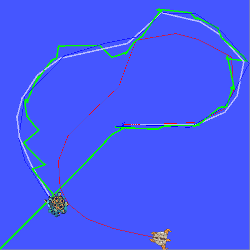
The first turtle, drawing a thick gray line, is our real turtlesim robot (the turtle’s shape is chosen randomly on creation, so it will vary from run to run). We will define two virtual sensors with a configurable frequency, systematic and random error: the position sensor will measure the turtle’s absolute position and orientation and is drawn with a thin blue line. The velocity sensor will measure the turtle’s linear and angular velocity and is drawn with a thin red line. The last turtle, drawing a thick green line, is robot_location’s estimate of the pose of the turtle in the map frame.
Of course, our turtlebot lives in a constrained 2D world. There is not that much sensor data to fuse with only one position and velocity sensor and our turtlebot’s infinite acceleration (it starts and stops immediately) is not a perfect fit for the motion model in the state estimator. But it’s good enough to get us up and running with the robot_localization package.
In this tutorial, we will only discuss the relevant parts of the demonstrator’s source code. You can find the full source code for this tutorial in our GitHub repository. If you are familiar with the concepts and code in the beginner level ROS and learning tf2 tutorials, understanding the rest of the source code should be a piece of cake.
We start by creating two virtual sensors for our turtlebot: an odometer, ‘measuring’ the linear and angular velocity of the turtlebot and a position sensor, ‘measuring’ the absolute position and orientation of the turtlebot.
Let’s start with the position sensor. You’ll find the full source code in the ros-ws/src/robot_localization directory. The include/robot_localization/positioning_system.hpp and src/sensors/positioning_system.cpp source files implement the position sensor class; the src/sensors/positioning_system_node.cpp starts a node for the sensor (accepting command-line parameters to configure the sensor).
The position sensor does nothing more than listening to the turtlesim/Pose messages on the turtle1/pose topic, caching the messages it receives and sending geometry_msgs/PoseWithCovarianceStamped messages (with the received position plus a systematic and random error) on the turtle1/sensors/pose topic.
Let’s have a look at the src/sensors/positioning_system.cpp source code.
  TurtlePositioningSystem::TurtlePositioningSystem(
      ros::NodeHandle node_handle, double frequency,
      double error_x_systematic, double error_x_random,
      double error_y_systematic, double error_y_random,
      double error_yaw_systematic, double error_yaw_random,
      bool visualize):
    node_handle_{node_handle},
    turtle_pose_subscriber_{
      node_handle_.subscribe("turtle1/pose", 16,
        &TurtlePositioningSystem::turtlePoseCallback, this)},
    turtle_pose_publisher_{
      node_handle_.advertise<geometry_msgs::PoseWithCovarianceStamped>(
        "turtle1/sensors/pose", 16)},
    frequency_{frequency},
    random_generator_{},
    random_distribution_x_{error_x_systematic, error_x_random},
    random_distribution_y_{error_y_systematic, error_y_random},
    random_distribution_yaw_{error_yaw_systematic, error_yaw_random},
    frame_sequence_{0},
    visualize_{visualize_},
    visualization_turtle_name_{""}
  {
    ;
  }
  TurtlePositioningSystem::~TurtlePositioningSystem() {
    ;
  }
The /turtle1/pose subscriber’s callback just caches the received pose. If the sensor is asked to visualize its measurements, it also calls the spawnAndConfigureVisualizationTurtle function to create a new turtle and set its line color to blue when receiving the first message.
void TurtlePositioningSystem::turtlePoseCallback(
      const turtlesim::PoseConstPtr & message) {
    cached_pose_timestamp_ = ros::Time::now();
    cached_pose_ = *message;
    // If this is the first message, initialize the visualization turtle.
    if(isVisualizationRequested() && !isVisualizationTurtleAvailable()) {
      spawnAndConfigureVisualizationTurtle(*message);
    }
  }
The spin function handles the main loop. At the requested measurement frequency, it retrieves the most recent pose received by the /turtle1/posesubscriber and distort it using the std::normal_distributions initialised in the constructor. This pose and an appropriate covariance matrix are packed in a geometry_msgs/PoseWithCovarianceStamped message. Note that the pose is expressed in the map frame (it’s an absolute, non-continuous measurement) and that we only use the fields required for a 2D pose estimation (we’ll ask the state estimator node to work in 2D mode in the launch file). Finally, this message is published on the /turtle1/sensors/pose topic. If we asked to visualize the measurement, move the visualization turtle to the measured location.
 void TurtlePositioningSystem::spin() {
    ros::Rate rate(frequency_);
    while(node_handle_.ok()) {
      ros::spinOnce();
      // Distort real pose to get a 'measurement'.
      auto measurement = cached_pose_;
      measurement.x += random_distribution_x_(random_generator_);
      measurement.y += random_distribution_y_(random_generator_);
      measurement.theta += random_distribution_yaw_(random_generator_);
      // Publish measurement.
      geometry_msgs::PoseWithCovarianceStamped current_pose;
      current_pose.header.seq = ++ frame_sequence_;
      current_pose.header.stamp = ros::Time::now();
      current_pose.header.frame_id = "map";
      current_pose.pose.pose.position.x = measurement.x;
      current_pose.pose.pose.position.y = measurement.y;
      current_pose.pose.pose.position.z = 0.;
      current_pose.pose.pose.orientation =
        tf::createQuaternionMsgFromRollPitchYaw(
          0., 0., measurement.theta);
      current_pose.pose.covariance = boost::array<double, 36>({
          std::pow(random_distribution_x_.mean()
                   + random_distribution_x_.stddev(), 2), 0., 0.,
            0., 0., 0.,
          0., std::pow(random_distribution_y_.mean()
                       + random_distribution_y_.stddev(), 2), 0.,
            0., 0., 0.,
          0., 0., 0., 0., 0., 0.,
          0., 0., 0., 0., 0., 0.,
          0., 0., 0., 0., 0., 0.,
          0., 0., 0., 0., 0.,
            std::pow(random_distribution_yaw_.mean()
                     + random_distribution_yaw_.stddev(), 2)});
      turtle_pose_publisher_.publish(current_pose);
      if(isVisualizationRequested() && isVisualizationTurtleAvailable()) {
        moveVisualizationTurtle(measurement);
      }
      // Sleep until we need to publish a new measurement.
      rate.sleep();
    }
  }
}
The code of the velocity sensor is very similar. The include/robot_localization/odometry.hpp and src/sensors/odometry.cppsource files implement the sensor class; the src/sensors/odometry_node.cppstarts a node for the sensor (accepting command-line parameters to configure the sensor).
The constructor, destructor and /turtle1/pose subscriber’s callback are almost identical to their position sensor counterparts. We calculate the angular velocity as the product of the linear velocity and the angular velocity error. This allows us to simulate a sensor with a systematic deviation from the straight line. This happens when we have a differential drive robot with different systematic errors on its wheel encoders. You can see that the turtlebot in the screenshot above (the one drawing a red line) has a clear deviation to the left. The velocity is measured (orientation and magnitude) relative to the robot, so it is expressed in the base_link frame (it could be transformed to a pose change in the odom frame, but the velocity (and acceleration when available) itself is expressed in the base_link frame).
We configure robot_localization via the launch file. First, we launch the turtlesim/turtlesim_node node to visualize the turtle, its sensor outputs and the position estimate and a turtlesim/turtle_teleop_key node to control the turtle using the keyboard.
<launch>
  <node pkg="turtlesim" type="turtlesim_node" name="turtlesim" />
  <node pkg="turtlesim" type="turtle_teleop_key"
        name="teleop"
        output="screen" />
The position sensor has a standard deviation of 0.2 units on the X and Y coordinates (the turtle’s playground above is 11 units wide and high) and 0.2 radians on the orientation of the turtle. The systematic error is unspecified and defaults to zero. It publishes a measurement every second.
  <node pkg="robot_localization_demo" type="positioning_system_node"
        name="turtle1_positioning_system_node"
        args="-f 1. -x 0.2 -y 0.2 -t 0.2 -v"
        output="screen" />
The velocity sensor publishes measurements at 10 Hz. It has a random error of 0.05 units/s (standard deviation) on the linear velocity and a systematic error of 0.02 times the linear velocity on the angular velocity (positive = counterclockwise).
  <node pkg="robot_localization_demo" type="odometry_node"
        name="turtle1_odometry_node"
        args="-f 20. -x 0.05 -X 0. -t 0. -T 0.02 -v"
        output="screen" />
As discussed earlier, we need two state estimator nodes: one for the odom → base_link transform and one for the map → odom transform. Let’s start with the first one. It updates its estimate at 10 Hz, we ask it to run in 2D mode, we explicitly ask to publish the tf2 transform too (although that is the default behavior), we specify the map, odom and base_link frames and by specifying the odom frame as the world_frame, we ask to estimate the odom → base_link transform.
We have one velocity sensor twist0 (all sensor topic names should start at 0 for the first sensor of a given type). We specify its topic (/turtle1/sensors/twist), we take the absolute value, not the difference between the current and the previous value (in general, if you have multiple similar sensors, all but one are used in differential mode, see the documentation for details) and it provides x˙, y˙ and yaw˙ measurements (we know our turtlebot can’t move sideways, so the y˙=0 measurement is a valid measurement). The true and false values are the parameters of the 15-dimensional state (x, y, z, roll, pitch, yaw, x˙, y˙, z˙, roll˙, pitch˙, yaw˙, x¨, y¨, z¨).
  <node pkg="robot_localization" type="ekf_localization_node"
        name="robot_localization_ekf_node_odom"
        clear_params="true">
    <param name="frequency" value="10." />
    <param name="sensor_timeout" value="0.2" />
    <param name="two_d_mode" value="true" />
    <param name="publish_tf" value="true" />
    <param name="map_frame" value="map" />
    <param name="odom_frame" value="odom" />
    <param name="base_link_frame" value="base_link" />
    <param name="world_frame" value="odom" />
    <remap from="odometry/filtered" to="odometry/filtered_twist" />
    <param name="twist0" value="turtle1/sensors/twist" />
    <param name="twist0_differential" value="false"/>
    <rosparam param="twist0_config">
      [false, false, false, false, false, false,
       true, true, false, false, false, true,
       false, false, false]</rosparam>
  </node>
The configuration of the map → odom state estimator node is similar, but it gets input not only from the velocity sensor, but also from the position sensor (providing x, y and yaw measurements).
  <node pkg="robot_localization" type="ekf_localization_node"
        name="robot_localization_ekf_node_map"
        clear_params="true">
    <param name="frequency" value="10" />
    <param name="sensor_timeout" value="0.2" />
    <param name="two_d_mode" value="true" />
    <param name="publish_tf" value="true" />
    <param name="map_frame" value="map" />
    <param name="odom_frame" value="odom" />
    <param name="base_link_frame" value="base_link" />
    <param name="world_frame" value="map" />
    <param name="twist0" value="turtle1/sensors/twist" />
    <rosparam param="twist0_config">
      [false, false, false, false, false, false,
       true, true, false, false, false, true,
       false, false, false]</rosparam>
    <param name="pose0" value="turtle1/sensors/pose" />
    <rosparam param="pose0_config">
      [true, true, false, false, false, true,
       false, false, false, false, false, false,
       false, false, false]</rosparam>
    <remap from="odometry/filtered" to="odometry/filtered_map"/>
  </node>
Finally, we add a helper node to show a turtle (drawing a thick green line) at the estimated position (map → … → base_link).
  <node pkg="robot_localization_demo" type="transformation_visualization_node"
        name="transformation_visualization_node" />
</launch>
First, source your preferred ROS version setup.bash (if you don’t do it in your ~/.bashrc already):
source /opt/ros/melodic/setup.bash
Then, go to the ros-ws directory in the tutorial root directory and build the tutorial code:
cd ~/…/robot-localization-demo/ros-ws
catkin_make
Finally, you are ready to run the demo. Source this workspace setup.bash and start the demo by using roslaunch:
source ./devel/setup.bash
roslaunch robot_localization_demo robot_localization_demo.launch
You can control the turtle using your keyboard’s arrow keys. Just make sure you have the input focus on the terminal running the roslaunch command (and the turtlesim/turtle_teleop_key node), not the turtlebot window itself.
You can play with the systematic and random errors of both sensors (have a look at the source code or launch the nodes with the –help option to see which command line parameters they support) and with the covariance they report. You can change the covariance in the source code (I implemented them in the source code to make them dependent on the systematic and random errors specified when starting the node) or override them in the launch file or a parameter file (have a look at the robot_localization package’s documentation for details).
After reading this tutorial, you should more or less know how robot_localization works. I didn’t show you all options of the robot_localization state estimator nodes and I didn’t show how to use the navsat_transform_node to integrate GPS data but you should have the background knowledge to read the robot_localization package documentation and know how it applies to your sensors.